They are used in various fields: from the evaluation of corporate performance and the quality of life in cities, to the efficiency of health systems. The goal is to provide a simple, interpretable and comparable measure. However, the apparent simplicity of these indices often masks arbitrary decisions, loss of information, and distortions in the resulting hierarchies.
One of the main problems is related to weight attribution: attributing a greater weight to one indicator than another implies a subjective preference. Furthermore, the synthesis in a single number forces a total ordering, even among units that differ on multiple dimensions in a non-comparable way, forcing a linear ordering through a single score leads to excessive simplifications and potentially misleading conclusions.
In light of these limitations, alternative approaches exist. Among these, POSETs (Partially Ordered Sets) offer a more faithful way to represent the complexity of multidimensional data.
Instead of synthesizing all the information in a number, POSETs are based on a partial dominance relationship: a unit dominates another if it is greater on all the dimensions considered. When this does not happen, the two units remain incomparable. The POSET approach allows us to represent the hierarchical structure implicit in the data without forcing comparisons where they are not logically justifiable. This makes it particularly useful in transparent decision-making contexts, where methodological coherence is preferable to forced simplification.
Starting from the theoretical foundations, we will build a practical example with a real dataset (Wine Quality dataset) and discuss result interpretation. We will see that, in the presence of conflicting dimensions, POSETs represent a robust and interpretable solution, preserving the original information without imposing an arbitrary ordering.
Theoretical foundations
To understand the POSET approach, it is necessary to start from some fundamental concepts of set theory and ordering. Unlike aggregative methods, which produce a total and forced ordering between units, POSET is based on the partial dominance relation, which allows us to recognize the incomparability among elements.
What is a partially ordered set?
A partially ordered set (POSET) is a couple (P, ≤), where
- P is a non-empty set (could be locations, companies, people, products, and so on)
- ≤ is a binary relationship on P that is characterized by three properties
- Reflexivity, each element is in relationship with itself (expressed as ∀ x ∈ P, x ≤ x)
- Antisymmetry, if two elements are related to each other in both directions, then they are the same (expressed as ∀ x, y ∈ P, ( x ≤ y ∧ y ≤ x) ⇒ x = y)
- Transitivity, if an element is related to a second, and the second with a third, then the first is in relation to the third (expressed as ∀ x, y, z ∈ P, (x ≤ y ∧ y ≤ z) ⇒ x ≤ z
In practical terms, an element x is said to dominate an element y (therefore x ≤ y) if it is greater or equal across all relevant dimensions, and strictly greater in at least one of them.
This structure is opposed to a total order, in which each pair of elements is comparable (for each x, y then x ≤ y or y ≤ x). The partial order, on the other hand, allows that some couples are incomparable, and this is one of its analytical forces.
Partial dominance relationship
In a multi-indicator context, the partial system is built by introducing a dominance relationship between vectors. Given two objects a = (a1, a2, …, an) and b = (b1, b2, …, bn) we can say that a ≤ b (a dominates b) if:
- for each i, ai ≤ bi (meaning that a is not the worst element among any dimensions)
- and that for at least one j, aj ≤ bj (meaning that a is strictly greater in at least one dimension compared to b)
This relationship builds a dominance matrix that represents which element dominates which other element in the dataset. If two objects do not satisfy the mutual criteria of dominance, they are incomparable.
For instance,
- if A = (7,5,6) and B = (8,5,7) then A ≤ B (because B is at least equal in each dimension and strictly greater in two of them)
- if C = (7,6,8) and D = (6,7,7) then C and D are incomparable because each one is greater than the other in at least one dimension but worse in the other.
This explicit incomparability is a key characteristic of POSETs: they preserve the original information without forcing a ranking. In many real applications, such as the quality evaluation of wine, city, or hospitals, incomparability is not a mistake, but a faithful representation of complexity.
How to build a POSET index
In our example we use the dataset winequality-red.csv, which contains 1599 red wines, each described by 11 chemical-physical variables and a quality score.
You can download the dataset here:
Wine Quality Dataset
Wine Quality Prediction – Classification Prediction
www.kaggle.com
The dataset’s license is CC0 1.0 Universal, meaning it can be downloaded and used without any specific permission.
Input variables are:
- fixed acidity
- volatile acidity
- citric acid
- residual sugar
- chlorides
- free sulfur dioxide
- total sulfur dioxide
- density
- pH
- sulphates
- alcohol
Output variable is quality (score between 0 and 10).
We can (and will) exclude variables in this analysis: the goal is to build a set of indicators consistent with the notion of “quality” and with shared directionality (higher values = better, or vice versa). For example, a high volatile acidity value is negative, while a high alcohol value is often associated with superior quality.
A rational choice may include:
- Alcohol (positive)
- Acidity volatile (negative)
- Sulphates (positive)
- Residual Sugar (positive up to a certain point, then neutral)
- Citric Acid (positive)
For POSET, it is important to standardize the semantic direction: if a variable has a negative effect, it must be transformed (e.g. -Volatile_acidity) before evaluating the dominance.
Construction of the dominance matrix
To build the partial dominance relationship between the observations (the wines), proceed as follows:
- Sample N observations from the dataset (for example, 20 wines for legibility purposes)
- Each wine is represented by a vector of m indicators
- The observation A dominates B occurs if A is greater or equal than B and at least one element is strictly greater.
Practical example in Python
The wine dataset is also present in Sklearn. We use Pandas to manage the dataset, Numpy for numerical operations and Networkx to build and view Hasse diagram
import pandas as pd
import numpy as np
import matplotlib.pyplot as plt
import networkx as nx
from sklearn.datasets import load_wine
from sklearn.preprocessing import MinMaxScaler
# load in the dataset
data = load_wine()
df = pd.DataFrame(data.data, columns=data.feature_names)
df['target'] = data.target
# let's select an arbitrary number of quantitative features
features = ['alcohol', 'malic_acid', 'color_intensity']
df_subset = df[features].copy()
# min max scaling for comparison purposes
scaler = MinMaxScaler()
df_norm = pd.DataFrame(scaler.fit_transform(df_subset), columns=features)
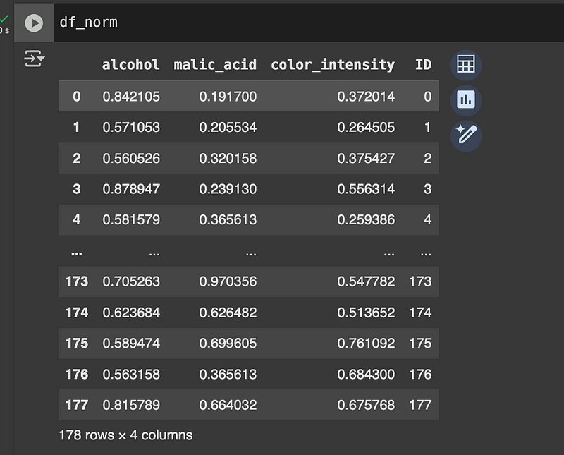
df_norm['ID'] = df_norm.indexEach line of the dataset represents a wine, described by 3 numerical characteristics. Let’s say that:
- Wine A dominates wine B if it has greater or equal values in all sizes, and strictly greater in at least one
This is just a partial system: you cannot always say if one wine is “better” than another, because maybe one has more alcohol but less color intensity.
We build the dominance matrix D, where d[i][j] = 1 if element i dominates j.
def is_dominant(a, b):
   """Returns True if a dominates b"""
   return np.all(a >= b) and np.any(a > b)

# dominance matrix
n = len(df_norm)
D = np.zeros((n, n), dtype=int)

for i in range(n):
   for j in range(n):
       if i != j:
           if is_dominant(df_norm.loc[i, features].values, df_norm.loc[j, features].values):
               D[i, j] = 1

# let's create a pandas dataframe
dominance_df = pd.DataFrame(D, index=df_norm['ID'], columns=df_norm['ID'])
print(dominance_df.iloc[:10, :10])


>>>
ID  0  1  2  3  4  5  6  7  8  9
ID
0   0  0  0  0  0  0  0  0  0  0
1   0  0  0  0  0  0  0  0  0  0
2   0  0  0  0  0  0  0  0  0  0
3   1  1  0  0  0  1  0  0  0  1
4   0  0  0  0  0  0  0  0  0  0
5   0  0  0  0  0  0  0  0  0  0
6   0  1  0  0  0  0  0  0  0  0
7   0  1  0  0  0  0  0  0  0  0
8   0  0  0  0  0  0  0  0  0  0
9   0  0  0  0  0  0  0  0  0  0
for each couple i, j, the matrix returns
- 1 if i dominates j
- else 0
For example, in line 3, you find values 1 in columns 0, 1, 5, 9. This means: element 3 dominates elements 0, 1, 5, 9.
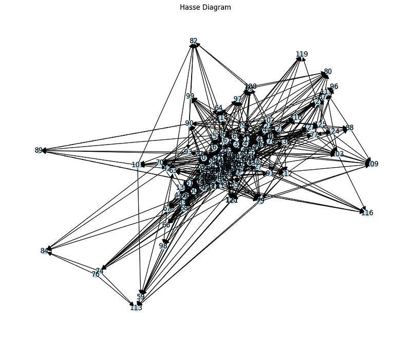
Building of Hasse diagram
We represent dominance relationships with an acliclic oriented graph. We reduce the relationships transitively to obtain the diagram of Hasse, which shows only direct dominances.
def transitive_reduction(D):
   G = nx.DiGraph()
   for i in range(len(D)):
       for j in range(len(D)):
           if D[i, j]:
               G.add_edge(i, j)

   G_reduced = nx.transitive_reduction(G)
   return G_reduced

# build the network with networkx
G = transitive_reduction(D)

# Visalization
plt.figure(figsize=(12, 10))
pos = nx.spring_layout(G, seed=42)
nx.draw(G, pos, with_labels=True, node_size=100, node_color='lightblue', arrowsize=15)
plt.title("Hasse Diagram")
plt.show()
Analysis of Incomparability
Let’s now see how many elements are incomparable to each other. Two units i and j are incomparable if neither dominates the other.
incomparable_pairs = []
for i in range(n):
   for j in range(i + 1, n):
       if D[i, j] == 0 and D[j, i] == 0:
           incomparable_pairs.append((i, j))

print(f"Number of incomparable couples: {len(incomparable_pairs)}")
print("Examples:")
print(incomparable_pairs[:10])

>>>
Number of incomparable couples: 8920
Examples:
[(0, 1), (0, 2), (0, 4), (0, 5), (0, 6), (0, 7), (0, 8), (0, 9), (0, 10), (0, 12)]
Comparison with a traditional synthetic ordering
If we used an aggregate index, we would get a forced total ordering. Let’s use the normalized mean for each wine as an example:
# Synthetic index calculation (average of the 3 variables)
df_norm['aggregated_index'] = df_norm[features].mean(axis=1)

# Total ordering
df_ordered = df_norm.sort_values(by='aggregated_index', ascending=False)
print("Top 5 wines according to aggregate index:")
print(df_ordered[['aggregated_index'] + features].head(5))

>>>
Top 5 wines according to aggregate index:
aggregated_index   alcohol  malic_acid  color_intensity
173          0.741133  0.705263    0.970356         0.547782
177          0.718530  0.815789    0.664032         0.675768
156          0.689005  0.739474    0.667984         0.659556
158          0.685608  0.871053    0.185771         1.000000
175          0.683390  0.589474    0.699605         0.761092
This example shows the conceptual and practical difference between POSET and synthetic ranking. With the aggregate index, each unit is forcedly ordered; with POSET, logical dominance relations are maintained, without introducing arbitrariness or information loss. The use of directed graphs also allows a clear visualization of partial hierarchy and incomparability between units.
Result interpretability
One of the most interesting aspects of the POSET approach is that not all units are comparable. Unlike a total ordering, where each element has a unique position, the partial ordering preserves the structural information of the data: some elements dominate, others are dominated, many are incomparable. This has important implications in terms of interpretability and decision making.
In the context of the example with the wines, the absence of a complete ordering implies that some wines are better on some dimensions and worse on others. For example, one wine could have a high alcohol content but a low color intensity, while another wine has the opposite. In these cases, there is no clear dominance, and the two wines are incomparable.
From a decision-making point of view, this information is valuable: forcing a total ranking masks these trade-offs and can lead to suboptimal choices.
Let’s check in the code how many nodes are maximal, that is, not dominated by any other, and how many are minimal, that is, do not dominate any other:
# Extract maximal nodes (no successors in the graph)
maximal_nodes = [node for node in G.nodes if G.out_degree(node) == 0]
# Extract minimal nodes (no predecessors)
minimal_nodes = [node for node in G.nodes if G.in_degree(node) == 0]

print(f"Number of maximal (non-dominated) wines: {len(maximal_nodes)}")
print(f"Number of minimal (all-dominated or incomparable) wines: {len(minimal_nodes)}")

>>>
Number of maximal (non-dominated) wines: 10
Number of minimal (all-dominated or incomparable) wines: 22
The high number of maximal nodes suggests that there are many valid alternatives without a clear hierarchy. This reflects the reality of multi-criteria systems, where there is not always a universally valid “best choice”.
Clusters of non-comparable wines
We can identify clusters of wines that are not comparable to each other. These are subgraphs in which the nodes are not connected by any dominance relation. We use networkx to identify the connected components in the associated undirected graph:
We can identify clusters of wines that are not comparable to each other. These are subgraphs in which the nodes are not connected by any dominance relation. We use networkx to identify the connected components in the associated undirected graph:
# Let's convert the directed graph into an undirected one
G_undirected = G.to_undirected()

# Find clusters of non-comparable nodes (connected components)
components = list(nx.connected_components(G_undirected))

# We filter only clusters with at least 3 elements
clusters = [c for c in components if len(c) >= 3]

print(f"Number of non-comparable wine clusters (≥3 units): {len(clusters)}")
print("Cluster example (up to 3)):")
for c in clusters[:3]:
   print(sorted(c))

>>>

Number of non-comparable wine clusters (≥3 units): 1
Cluster example (up to 3)):
[0, 1, 2, 3, 4, 5, 6, 7, 8, 9, 10, ...]
These groups represent regions of multidimensional space in which units are equivalent in terms of dominance: there is no objective way to say that one wine is “better” than another, unless we introduce an external criterion.
Hasse diagram with focus on maximals
To better visualize the structure of the sorting, we can highlight the maximal nodes (optimal choices) in the Hasse diagram:
node_colors = ['skyblue' if node in maximal_nodes else 'lightgrey' for node in G.nodes]

plt.figure(figsize=(12, 10))
pos = nx.spring_layout(G, seed=42)
nx.draw(G, pos, with_labels=True, node_size=600, node_color=node_colors, arrowsize=15)
plt.title("Maximal nodes highlighted (not dominated)")
plt.show()
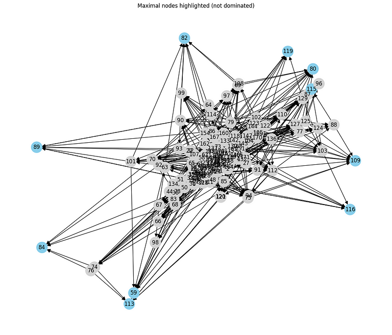
In real scenarios, these maximal nodes would correspond to non-dominated solutions, i.e. the best options from a Pareto-efficiency perspective. The decision maker could choose one of these based on personal preferences, external constraints or other qualitative criteria.
Unremovable trade-offs
Let’s take a concrete example to show what happens when two wines are incomparable:
id1, id2 = incomparable_pairs[0]
print(f"Comparison between wine {id1} and {id2}:")

v1 = df_norm.loc[id1, features]
v2 = df_norm.loc[id2, features]

comparison_df = pd.DataFrame({'Wine A': v1, 'Wine B': v2})
comparison_df['Dominance'] = ['A > B' if a > b else ('A < B' if a < b else '=') for a, b in zip(v1, v2)]

print(comparison_df)

>>>
Comparison between wine 0 and 1:
                  Wine A    Wine B Dominance
alcohol          0.842105  0.571053     A > B
malic_acid       0.191700  0.205534     A < B
color_intensity  0.372014  0.264505     A > B
This output clearly shows that neither wine is superior on all dimensions. If we used an aggregate index (such as an average), one of the two would be artificially declared “better”, erasing the information about the conflict between dimensions.
Chart interpretation
It is important to know that a POSET is a descriptive, not a prescriptive, tool. It does not suggest an automatic decision, but rather makes explicit the structure of the relationships between alternatives. Cases of incomparability are not a limit, but a feature of the system: they represent legitimate uncertainty, plurality of criteria and variety of solutions.
In decision-making areas (policy, multi-objective selection, comparative evaluation), this interpretation promotes transparency and responsibility of choices, avoiding simplified and arbitrary rankings.
Pros and Cons of POSETs
The POSET approach has a number of important advantages over traditional synthetic indices, but it is not without limitations. Understanding these is essential to deciding when to adopt a partial ordering in multidimensional analysis projects.
Pros
- Transparency: POSET does not require subjective weights or arbitrary aggregations. Dominance relationships are determined solely by the data.
- Logical coherence: A dominance relationship is defined only when there is superiority on all dimensions. This avoids forced comparisons between elements that excel in different aspects.
- Robustness: Conclusions are less sensitive to data scale or transformation, provided that the relative ordering of variables is maintained.
- Identifying non-dominated solutions: Maximal nodes in the graph represent Pareto-optimal choices, useful in multi-objective decision-making contexts.
- Making incomparability explicit: Partial sorting makes trade-offs visible and promotes a more realistic evaluation of alternatives.
Cons
- No single ranking: In some contexts (e.g., competitions, rankings), a total ordering is required. POSET does not automatically provide a winner.
- Computational complexity: For very large datasets, dominance matrix construction and transitive reduction can become expensive.
- Communication challenges: for non-expert users, interpreting a Hasse graph may be less immediate than a numerical ranking.
- Dependence on preliminary choices: The selection of variables influences the structure of the sort. An unbalanced choice can mask or exaggerate the incomparability.
Conclusions
The POSET approach offers a powerful alternative perspective for the analysis of multidimensional data, avoiding the simplifications imposed by aggregate indices. Instead of forcing a total ordering, POSETs preserve information complexity, showing clear cases of dominance and incomparability.
This methodology is particularly useful when:
- indicators describe different and potentially conflicting aspects (e.g. efficiency vs. equity);
- you want to explore non-dominated solutions, in a Pareto perspective;
- you need to ensure transparency in the decision-making process.
However, it is not always the best choice. In contexts where a unique ranking or automated decisions are required, it may be less practical.
The use of POSETs should be considered as an exploratory phase or complementary tool to aggregative methods, to identify ambiguities, non-comparable clusters, and equivalent alternatives.